interp

Name

interp — cubic spline evaluation function

Calling Sequence

[yp [,yp1 [,yp2 [,yp3]]]]=interp(xp, x, y, d [, out_mode])

Parameters

xp: real vector or matrix
x,y,d: real vectors of the same size defining a cubic spline or sub-spline function (called s in the following)
out_mode: (optional) string defining the evaluation of s outside the [x1,xn] interval
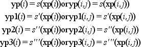
yp: vector or matrix of same size than xp, elementwise evaluation of s on xp (yp(i)=s(xp(i) or yp(i,j)=s(xp(i,j))
yp1, yp2, yp3: vectors (or matrices) of same size than xp, elementwise evaluation of the successive derivatives of s on xp

Description

Given three vectors (x,y,d) defining a spline or sub-spline function (see splin) with yi=s(xi), di = s'(xi) this function evaluates s (and s', s'', s''' if needed) at xp(i) :

The out_mode parameter set the evaluation rule for extrapolation, i.e. for xp(i) not in [x1,xn] :

"by_zero": an extrapolation by zero is done
"by_nan": extrapolation by Nan
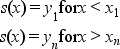
"C0": the extrapolation is defined as follows :
"natural": the extrapolation is defined as follows (p_i being the polynomial defining s on [x_i,x_{i+1}]) :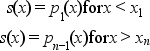
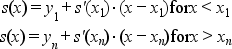
"linear": the extrapolation is defined as follows :
"periodic": s is extended by periodicity.

Examples

 
// see the examples of splin and lsq_splin

// an example showing C2 and C1 continuity of spline and subspline
a = -8; b = 8;
x = linspace(a,b,20)';
y = sinc(x);
dk = splin(x,y);  // not_a_knot
df = splin(x,y, "fast");
xx = linspace(a,b,800)';
[yyk, yy1k, yy2k] = interp(xx, x, y, dk); 
[yyf, yy1f, yy2f] = interp(xx, x, y, df); 
clf()
subplot(3,1,1)
plot2d(xx, [yyk yyf])
plot2d(x, y, style=-9)
legends(["not_a_knot spline","fast sub-spline","interpolation points"],...
        [1 2 -9], "ur",%f)
xtitle("spline interpolation")
subplot(3,1,2)
plot2d(xx, [yy1k yy1f])
legends(["not_a_knot spline","fast sub-spline"], [1 2], "ur",%f)
xtitle("spline interpolation (derivatives)")
subplot(3,1,3)
plot2d(xx, [yy2k yy2f])
legends(["not_a_knot spline","fast sub-spline"], [1 2], "lr",%f)
xtitle("spline interpolation (second derivatives)")

// here is an example showing the different extrapolation possibilities
x = linspace(0,1,11)';
y = cosh(x-0.5);
d = splin(x,y);
xx = linspace(-0.5,1.5,401)';
yy0 = interp(xx,x,y,d,"C0");
yy1 = interp(xx,x,y,d,"linear");
yy2 = interp(xx,x,y,d,"natural");
yy3 = interp(xx,x,y,d,"periodic");  
clf()
plot2d(xx,[yy0 yy1 yy2 yy3],style=2:5,frameflag=2,leg="C0@linear@natural@periodic")
xtitle(" different way to evaluate a spline outside its domain")

Authors

B. Pincon