Parameters

Description

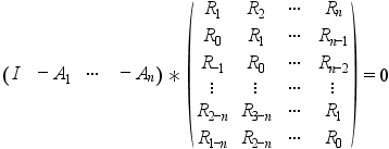
function which solves recursively on n the following Toeplitz system (normal equations)

where {Rk;k=1:nlag} is the sequence of nlag empirical covariances

Examples

 
//We use the 'levin' macro for solving the normal equations 
//on two examples: a one-dimensional and a two-dimensional process.
//We need the covariance sequence of the stochastic process.
//This example may usefully be compared with the results from 
//the 'phc' macro (see the corresponding help and example in it)
//
//
//1) A one-dimensional process
//   -------------------------
//
//We generate the process defined by two sinusoids (1Hz and 2 Hz) 
//in additive Gaussian noise (this is the observed process); 
//the simulated process is sampled at 10 Hz (step 0.1 in t, underafter).

t1=0:.1:100;rand('normal');
y1=sin(2*%pi*t1)+sin(2*%pi*2*t1);y1=y1+rand(y1);plot(t1,y1);

//covariance of y1

nlag=128;
c1=corr(y1,nlag);
c1=c1';//c1 needs to be given columnwise (see the section PARAMETERS of this help)

//compute the filter for a maximum order of n=10
//la is a list-type variable each element of which 
//containing the filters of order ranging from 1 to n; (try varying n)
//in the d-dimensional case this is a matrix polynomial (square, d X d)
//sig gives, the same way, the mean-square error

n=15;
[la1,sig1]=levin(n,c1);

//verify that the roots of 'la' contain the 
//frequency spectrum of the observed process y
//(remember that y is sampled -in our example 
//at 10Hz (T=0.1s) so that we need to retrieve 
//the original frequencies (1Hz and 2 Hz) through 
//the log and correct scaling by the frequency sampling)
//we verify this for each filter order

for i=1:n, s1=roots(la1(i));s1=log(s1)/2/%pi/.1;

//now we get the estimated poles (sorted, positive ones only !)

s1=gsort(imag(s1));s1=s1(1:i/2);end;

//the last two frequencies are the ones really present in the observed 
//process ---> the others are "artifacts" coming from the used model size.
//This is related to the rather difficult problem of order estimation.
//
//2) A 2-dimensional process 
//   -----------------------
//(4 frequencies 1, 2, 3, and 4 Hz, sampled at 0.1 Hz :
//   |y_1|        y_1=sin(2*Pi*t)+sin(2*Pi*2*t)+Gaussian noise
// y=|   | with : 
//   |y_2|        y_2=sin(2*Pi*3*t)+sin(2*Pi*4*t)+Gaussian noise

d=2;dt=0.1;
nlag=64;
t2=0:2*%pi*dt:100;
y2=[sin(t2)+sin(2*t2)+rand(t2);sin(3*t2)+sin(4*t2)+rand(t2)];
c2=[];
for j=1:2, for k=1:2, c2=[c2;corr(y2(k,:),y2(j,:),nlag)];end;end;
c2=matrix(c2,2,128);cov=[];
for j=1:64,cov=[cov;c2(:,(j-1)*d+1:j*d)];end;//covar. columnwise
c2=cov;

//in the multidimensional case, we have to compute the 
//roots of the determinant of the matrix polynomial 
//(easy in the 2-dimensional case but tricky if d>=3 !). 
//We just do that here for the maximum desired 
//filter order (n); mp is the matrix polynomial of degree n

[la2,sig2]=levin(n,c2);
mp=la2(n);determinant=mp(1,1)*mp(2,2)-mp(1,2)*mp(2,1);
s2=roots(determinant);s2=log(s2)/2/%pi/0.1;//same trick as above for 1D process
s2=gsort(imag(s2));s2=s2(1:d*n/2);//just the positive ones !

//There the order estimation problem is seen to be much more difficult !
//many artifacts ! The 4 frequencies are in the estimated spectrum 
//but beneath many non relevant others.
 

See Also

Authors

G. Le Vey